First, we need to ensure the InvariantRing package is loaded.
Subsection3.1What is Invariant Theory?
Let a group \(G\) act linearly on a vector space \(V\) over a field \(K\text{.}\) This action extends to the polynomial ring \(R = K[V] = K[x_1, \dots, x_n]\) by \((g \cdot f)(x) = f(g^{-1} \cdot x)\) for \(g \in G, f \in R\text{.}\) A polynomial \(f\) is an invariant if \(g \cdot f = f\) for all \(g \in G\text{.}\) The set of all such invariant polynomials forms a subring \(R^G \subseteq R\text{,}\) called the ring of invariants.
A very first example is the invariants of the symmetric group known to Newton. Let’s generate the group \(\mathcal S_4\) using the permutations \(2134\) and \(2341\text{.}\) This is the well-celebrated fact that \(\mathcal S_n\) can be minimally generated by a simple transposition and an \(n\)-cycle.
These are our old friends, symmetric polynomials. How about the alternating group \(\mathcal A_4\text{?}\)
Indeed, the \(\mathcal A_n\) invariants are generated by the elementary symmetrics and the Vandemonde determinant.
A set of homogeneous invariants \(f_1, \dots, f_n \in K[V]^G\) (where \(n = \dim(V)\)) forms a homogeneous system of parameters if they are algebraically independent and the invariant ring \(K[V]^G\) is a finitely generated module over the polynomial subalgebra
\begin{equation*}
A := K[f_1, \dots, f_n].
\end{equation*}
These \(f_i\) are then called primary invariants. Since \(K[V]^G\) is Cohen-Macaulay when \(G\) is linearly reductive (Theorem 2.6.5), it is actually a free module over \(A\) (Proposition 2.6.3). This means
\begin{equation*}
K[V]^G = \bigoplus_{j=1}^s A \cdot g_j
\end{equation*}
for some homogeneous invariants \(g_1, \dots, g_s \in K[V]^G\text{.}\) These \(g_j\) (including \(g_1=1\)) are called secondary invariants. Together, the primary and secondary invariants generate \(K[V]^G\) as a \(K\)-algebra. Let’s try this for \(\mathcal A_4\text{.}\)
Subsection3.2Diagonal Actions and Quotient Singularities
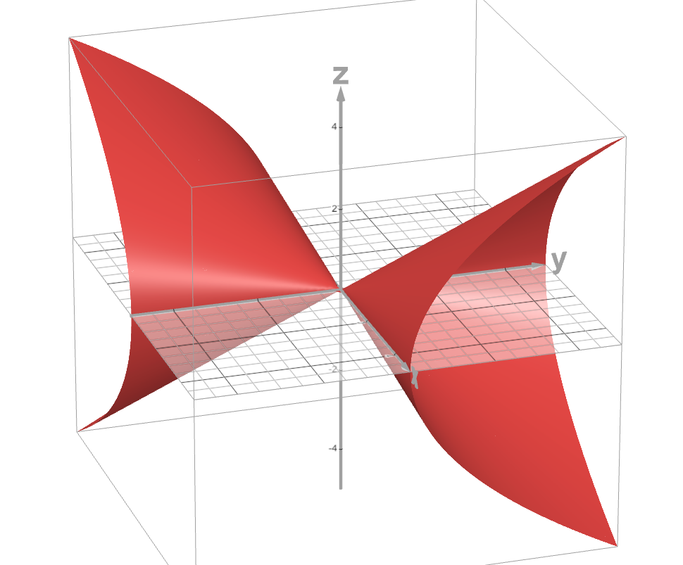
Now, let’s do some geometry. Consider the cyclic group \(C_2\) acting on the affine plane \(\mathbb A^2\) by \(-1\cdot(x,y) = (-x,-y)\text{.}\) We want to understand the quotient \(\mathbb A^2 / C_2\text{.}\) Taking quotients contravariantly corresponds to taking the ring of invariants \(k[x,y]^{C_2}\text{.}\)
... so \(k[x,y]^{C_2} = k[x^2, xy, y^2] \cong \frac{k[X,Y,Z]}{Z^2 - XY}\) is the coordinate ring for the quadric cone!
Figure3.1.
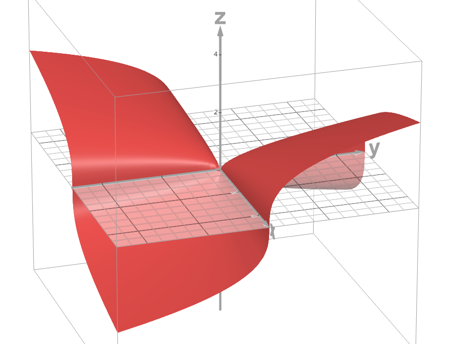
Next, consider the cyclic group \(C_3\) acting on the affine plane \(\mathbb A^2\) by \(-1\cdot(x,y) = (\zeta_3 x,\zeta_3^2 y)\text{,}\) where \(\zeta_3\) is a 3rd root of unity.
... so \(k[x,y]^{C_3} = k[x^3, xy, y^3] \cong \frac{k[X,Y,Z]}{Z^3 - XY}\) is a rational double point of type \(A_2\text{.}\) TODO: Calculate the invariants for ADE singularities.
Figure3.2.
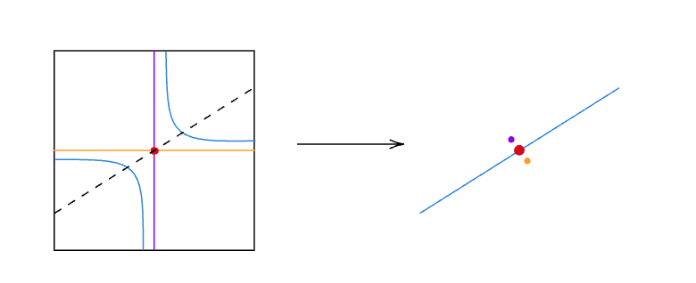
Both of the above actions live inside the action of \(\mathbb G_m\) on \(\mathbb A^2\) of bidegree \((1,-1)\text{.}\) What are its invariants?
We see that \(xy\) is the only global invariant function of this action. The GIT quotient is therefore \(\operatorname{Spec} k[xy]\) which is the affine line. This can be seen from the following doodle of the orbits:
Figure3.3.
There are 3 kinds of orbits: the hyperbola \(\{xy = a \mid a \neq 0\}\text{,}\) the axes, and the origin. The hyperbola form an \(\mathbb A^1 - 0\)-worth of closed orbits. The axes are the non-closed orbits, and the origin is the ’stacky point’. The GIT quotient crashes the latter 3 into one single point.
Subsection3.3Linearly Reductive Groups and Hilbert’s Finiteness Theorem
Recall that a rational representation of a linear algebraic group \(G\) is a representation \(V\) such that the \(G\) action is regular when \(V\) is viewed as an affine space. A linear algebraic group \(G\) is linearly reductive if for every rational representation \(V\) and every \(v \in V^G - 0\text{,}\) there exists a linear invariant function \(f \in\left(V^*\right)^G\) such that \(f(v) \neq 0\text{.}\)
Example3.4.(2.2.18) Non-reductive action..
Let \(\mathbb{G}_a=K\) be the additive group. We define a regular action on \(K^2\) by
The invariant ring \(K[x, y]^{\mathbb{G}_a}\) is equal to \(K[y]\text{.}\) If \(v \in K \times\{0\}=\left(K^2\right)^{\mathbb{G}_a}\text{,}\) then every invariant vanishes on \(v\text{.}\) The group \(\mathbb{G}_a\) is therefore not geometrically reductive.
Subsection3.4The Reynolds Operator and a Proof of Hilbert’s Theorem
Subsubsection3.4.1The Reynolds Operator
For a linearly reductive group \(G\) acting on an affine \(G\)-variety \(X\text{,}\) the Reynolds operator\(\mathcal{R}: K[X] \to K[X]^G\) is a \(K[X]^G\)-module homomorphism that is also a projection onto the invariant ring. This means it satisfies:
\(\mathcal{R}(f) = f\) for all \(f \in K[X]^G\) (Projection property).
\(\mathcal{R}(\sigma \cdot f) = \mathcal{R}(f)\) for all \(f \in K[X]\) and \(\sigma \in G\) (G-invariance).
\(\mathcal{R}(fh) = f \mathcal{R}(h)\) for all \(f \in K[X]^G\) and \(h \in K[X]\) (Module homomorphism property).
For a finite group \(G\) where \(|G|\) is invertible in \(K\text{,}\) the Reynolds operator is simply averaging over the group: \(\mathcal{R}(f) = \frac{1}{|G|} \sum_{\sigma \in G} \sigma \cdot f\text{.}\) For other linearly reductive groups (like \(GL_n(K)\) or \(SL_n(K)\) in characteristic 0), averaging with the Haar measure provides a good heuristic. Reynolds operators for infinite groups are usually defined via Casimir operators; for GL_n, SL_n in particular, one may use Cayley’s Omega Process (cf. Chapter 4 of DK15).
Subsubsection3.4.2Hilbert’s Proof of Finiteness (Theorem 2.2.10)
Proof Sketch:
Let \(K[V]^G_+\) be the set of all homogeneous invariants of positive degree. Consider the ideal \(I := K[V]^G_+ \cdot K[V]\) in the polynomial ring \(K[V]\text{.}\) This ideal is generated by all homogeneous invariants of positive degree.
By Hilbert’s Basis Theorem, the polynomial ring \(K[V]\) is Noetherian. Therefore, the ideal \(I\) is finitely generated. We can choose a finite set of homogeneous G-invariants \(f_1, \dots, f_r \in K[V]^G_+\) such that \(I = (f_1, \dots, f_r)K[V]\text{.}\) (The text notes this choice is justified by Proposition 4.1.1, but Hilbert’s original argument relies on \(I\) being finitely generated by some polynomials \(h_i \in K[V]\text{,}\) then \(\mathcal{R}(h_i)\) yield invariant generators for \(I\) as an ideal in \(K[V]\) generated by invariants).
We claim that these invariants \(f_1, \dots, f_r\) actually generate the entire invariant ring \(K[V]^G\) as a \(K\)-algebra. We prove this by induction on the degree \(d\) of a homogeneous invariant \(h \in K[V]^G\text{.}\)
Base case: If \(d=0\text{,}\) then \(h \in K\text{,}\) which is certainly generated by \(f_1, \dots, f_r\) (or by 1 if one includes constant invariants).
Inductive step: Assume all homogeneous invariants of degree less than \(d\) are in \(K[f_1, \dots, f_r]\text{.}\) Let \(h \in K[V]^G\) be homogeneous of degree \(d > 0\text{.}\) Since \(h \in I\text{,}\) we can write \(h = \sum_{i=1}^r a_i f_i\) for some \(a_i \in K[V]\text{.}\) We can choose these \(a_i\) to be homogeneous such that \(\deg(a_i) = d - \deg(f_i)\text{.}\) Since \(\deg(f_i) > 0\text{,}\) we have \(\deg(a_i) < d\text{.}\)
Apply the Reynolds operator \(\mathcal{R}\) to the equation \(h = \sum a_i f_i\text{.}\) Since \(h\) is invariant, \(\mathcal{R}(h) = h\text{.}\) Since each \(f_i\) is invariant and \(\mathcal{R}\) is a \(K[V]^G\)-module homomorphism (Corollary 2.2.7b), we get:
Each \(\mathcal{R}(a_i)\) is a homogeneous G-invariant. Its degree is \(\deg(a_i) = d - \deg(f_i) < d\text{.}\) By the induction hypothesis, each \(\mathcal{R}(a_i)\) belongs to \(K[f_1, \dots, f_r]\text{.}\) Therefore, \(h = \sum \mathcal{R}(a_i) f_i\) also belongs to \(K[f_1, \dots, f_r]\text{.}\)
By induction, all homogeneous invariants are in \(K[f_1, \dots, f_r]\text{.}\) Since \(K[V]^G\) is a graded ring generated by its homogeneous elements, it follows that \(K[V]^G = K[f_1, \dots, f_r]\text{,}\) and thus \(K[V]^G\) is finitely generated.
Existence of the Reynolds operator and the Noetherian property are key in this proof. The ideal of invariants \(I = K[V]^G_+ K[V]\) is often called the Hilbert ideal.
Subsection3.5\(SL_n\)-Invariants
In this final section, let’s try to calculate some \(SL_n\)-invariants. Take the standard representation of \(SL_2\) on a \(2\)-dimensional vector space \(V\text{.}\) Suppose the dual \(V^\vee\) has basis \(x,y\text{.}\) The symmetric power \(\operatorname{Sym}^2 V^\vee\) is another \(SL_2\)-representation, where elements are binary quadratic forms, where a generic element looks like \(Ax^2 + Bxy + Cy^2\text{.}\) Induced by \begin{pmatrix}a & b \\ c & d \end{pmatrix}\cdot (x,y) = (ax + by, cx+ dy),\(SL_2\) acts quadratically on the 3 coeffiecients.
To start off, let’s define the coordinate ring of \(SL_2\text{.}\)
Next, here’s a neat way to extract the action on binary forms.
The defining ideal of the group, the action matrix, plus another ring for the 3 coefficients of a binary form is enough to define the action.
What are its invariants?
... the discriminant of a quadratic equation!
We can run the same Spiel for binary cubic forms. This time, the generic form \(Ax^3 + Bx^2y + Cxy^2 + Dy^3\) has 4 coefficients.
This is the degree 4 discriminant for cubic equations.
How about ternary cubic forms \(A_0x^3 + A_1 y^3 + A_2z^3 + \cdots + A_9 xyz\text{?}\) Recall that these correspond to plane cubic curves. We could do the same as above, but the program won’t terminate in a reasonable amount of time. We could instead use a resultant (cf. DK15 Section 2.1).
This is the famous discriminant of an elliptic curve! It is an irreducible polynomial of degree \(12\) in \(10\) variables, with \(2040\) terms. It is closely related to the Eisenstein series \(E_4, E_6\text{.}\) Geometrically, this means that the locus of singular plane cubics in the parameter space \(\mathbb P^9\) is a degree \(12\) hypersurface.
Subsection3.6Some notes on the algorithms
The algorithm currently implemented for computing linearly reductive invariants leverages elimination theory and the properties of the Hilbert ideal.
The core idea of the algorithm (Algorithm 4.1.9 in Derksen & Kemper, "Computational Invariant Theory") can be summarized in the following high-level steps:
Represent the Group and Action: The group \(G\) is described as an affine variety (e.g., by equations in \(K[z_1, \dots, z_l]\)), and the representation \(G \to GL(V)\) is given by a matrix \(A_{\text{action}}(z)\) whose entries are polynomials in the \(z_i\text{.}\)
Construct the Graph Ideal (\(\mathfrak{b}\)): An ideal \(I_{\Gamma}\) is formed in a larger polynomial ring \(K[x_1,\dots,x_n, y_1,\dots,y_n, z_1,\dots,z_l]\text{.}\) This ideal defines the graph of the action, encoding pairs \((v, \sigma \cdot v)\) for \(v \in V, \sigma \in G\text{.}\) Specifically, it’s generated by:
The defining equations of \(G\) (in variables \(z_j\)).
The equations \(y_i - \sum_k (A_{\text{action}}(z))_{ik} x_k = 0\) for \(i=1,\dots,n\text{,}\) which relate the coordinates \(y\) of \(\sigma \cdot x\) to the coordinates \(x\) of \(v\) and group parameters \(z\text{.}\)
Eliminate Group Variables: A Gröbner basis \(\mathcal{G}\) of \(I_{\Gamma}\) is computed with respect to a monomial order that eliminates the group variables \(z_j\text{.}\) The elements of \(\mathcal{G}\) that lie in \(K[x,y]\) form a Gröbner basis for the ideal \(\mathfrak{b} = I_{\Gamma} \cap K[x,y]\text{.}\) This ideal \(\mathfrak{b}\) is the vanishing ideal of the closure of the set \(\{(v, \sigma \cdot v) | v \in V, \sigma \in G\}\text{.}\)
Compute Generators for the Hilbert Ideal: If \(\{f_j(x,y)\}\) are homogeneous generators of \(\mathfrak{b}\text{,}\) then the polynomials \(\{f_j(x,0)\}\) generate the Hilbert ideal\(I_H = K[V]^G_+ K[V]\) in \(K[x] = K[V]\text{.}\)
Working around the Reynolds operator: By Proposition 4.1.1 in Derksen & Kemper, if \(I_H = (h_1(x), \dots, h_s(x))\) where \(h_k\) are homogeneous (not necessarily invariant), then \(K[V]^G = K[\mathcal{R}(h_1), \dots, \mathcal{R}(h_s)]\text{,}\) where \(\mathcal{R}\) is the Reynolds operator. The invariants(LinearlyReductiveAction) method computes the Hilbert ideal first using hilbertIdeal then finds invariant generators degree by degree.
There is ongoing work to implement more direct and potentially efficient methods for constructing the Reynolds operator itself. Two classical approaches being explored are:
Via the Casimir Operator: For a connected semi-simple Lie group \(G\text{,}\) the Casimir operator is a specific element in the center of the universal enveloping algebra of its Lie algebra \(\mathfrak{g}\text{.}\) It commutes with the action of \(G\) on any representation and acts as a scalar on irreducible representations. The Reynolds operator can be constructed using the Casimir operator (see Algorithm 4.5.19/4.5.20 in Derksen & Kemper).
Via Cayley’s Omega Process: For \(GL_n(K)\) and \(SL_n(K)\text{,}\) Cayley’s \(\Omega\)-process produces invariants via explicit differential operators -- the \(\Omega\)-operator \(\det(\frac{\partial}{\partial z_{ij}})\text{,}\) where \(z_{ij}\) are matrix entries. The Reynolds operator can be expressed in terms of iterates of the \(\Omega\)-operator and powers of its determinant (Propositions 4.5.27 and 4.5.28 in Derksen & Kemper).
That it! Hope you had a lot of fun! --Michael R. Zeng